
Overview of the pipeline functions
Step 1 data analysis; From raw data to essential protein overview
SATAY experiments need to be sequenced which results in a FASTQ file. The sequence reads from this file needs to be aligned to create a SAM file (and/or the compressed {bash}ary equivalent BAM file). Using the BAM file, the number of transposons can be determined for each insertion location.
Raw data (.FASTQ file) discussed in the paper of Michel et.al. 2017 can be found at [https://www.ebi.ac.uk/arrayexpress/experiments/E-MTAB-4885/samples/].
Workflow
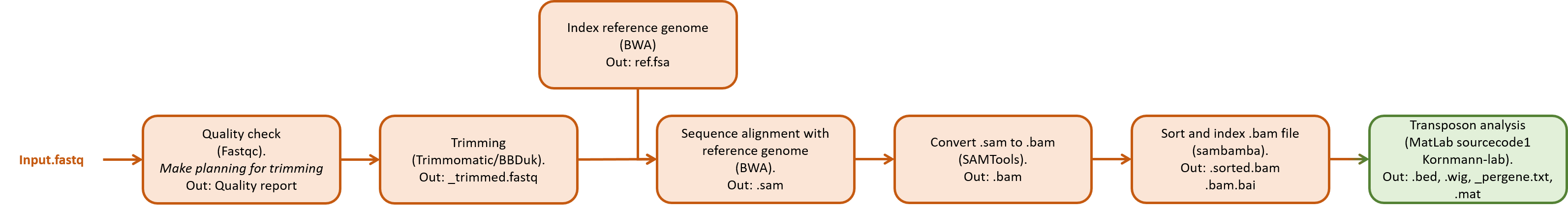
The results from the sequencing is typically represented in FASTA or FASTQ format. This needs to be aligned according to a reference sequence to create a SAM and BAM file. Before alignment, the data needs to be checked for quality and possibly trimmed to remove unwanted and unnecessary sequences. When the location of the reads relative to a reference sequence are known, the insertion sites of the transposons can be determined. With this, a visualization can be made that shows the number of transposon insertions per gene.
In the description given in this document, it is chosen to do the quality checking and the trimming in windows and the alignment of the reads with a reference genome in a virtual machine running Linux. It is possible to do the quality checking and trimming in Linux as well or to do the whole process in windows. To do quality checking and/or trimming in Linux requires more memory of the Linux machine since both the raw sequencing data needs to be stored and the trimming needs to be stored (both which can be relatively large files). Since a virtual machine is used, both the computation power and the amount of storage is limited, and therefore it chosen to do the trimming on the main windows computer (this problem would not exists if a computer is used running on Linux, for example a computer with an alternative startup disc running Linux). Sequence alignment can be done on Windows machines (e.g. using BBmap), but this is not ideal as many software tools are designed for Unix based computer systems (i.e. Mac or Linux). Also, many tools related to sequence alignment (e.g. converting .sam files to .bam and sorting and indexing the bam files) are done with tools not designed to be used in windows, hence this is performed in Linux.
An overview of the different processing steps are shown in the figure below.
A short overview is given for different software tools that can be used for processing and analyzing the data. Next, a step-by-step tutorial is given as an example how to process the data. Most of this is done using command line based tools.
An overview of the different steps including some software that can handle this is shown here:
Checking the raw FASTA or FASTQ data can be done using the (FASTQC) software (Windows, Linux, Mac. Requires Java). This gives a quality report (see accompanying tutorial) for the sequence reads and can be run non-interactively using the command line.
Based on the quality report, the data needs to be trimmed to remove any unwanted sequences. This can be done with for example (FASTX) (Linux, Mac) or (Trimmomatic) (Windows,requires Java). An easy graphical user interface that com{bash}es the FASTQC and Trimmomatic is (123FASTQ). Also BBDuk can be used for trimming (which belongs to BBMap).
The trimmed sequence reads need to be aligned using a reference sequence, for example the S. Cerevisiae S288C Ref64-2-1 reference sequence or the W303 reference sequence from SGD. Aligning can be done, for example, using (SnapGene) (Windows, Linux, Mac. This does not import large files and is therefore not suitable for whole genome sequencing), (BBMap) (Linux, Mac, Windows (seems to give problems when installing on windows machines), might be possible to integrate it in Python, (BWA) (Linux, Mac), (Bowtie2) (Linux, Mac) or (ClustalOmega) (Windows, Linux, Mac). This step might require defining scores for matches, mismatches, gaps and insertions of nucleotides.
After aligning, the data needs to be converted to SAM and BAM formats for easier processing hereafter. This requires (SAMtools) (Linux, Mac) or (GATK) (Linux, Mac). Conversion from SAM to BAM can also be done in Matlab if preferred using the ‘BioMap’ function.
Using the BAM file with the aligned sequence reads, the transposon insertion sites can be determined using the Matlab script given by Benoit Kornmann Lab (including the name.mat and yeastGFF.mat files). The results from this step are three files (a .txt file, a .bed file and a .wig file) that can be used for visualization.
If more processing is required, (Picard) (Linux, Mac) might be useful, as well as (GATK) (Linux, Mac). Visualization of the genomic dataset can be done using (IGV) (Windows, Linux, Mac) or SAMtools’ tview function. Also (sambamba) (Linux, Mac) can be used, especially for sorting and indexing the bam files.
Creating transposon insertion maps for the genome (see the satay users website) and comparison essential genes between different genetic backgrounds using Venn diagrams, customized software needs to be created.
Quality checking of the sequencing reads; FASTQC (0.11.9)
FASTQC creates a report for the quality of sequencing data. The input should be a fastq (both zipped and unzipped), sam or bam file (it can handle multiple files at once). The program does not need to be installed, but after downloading only requires to be unzipped. FASTQC can be ran as an interactive program (i.e. using a GUI) or non-interactively using the command line options.
If using interactively, open the ‘run_fastqc.bat’ file in the FASTQC folder and load a file to be checked. Alternatively using the 123FASTQ (version 1.1) program, open this and use the ‘Quality Check’ menu on the right. The advantage of using 123FASTQ is that it can also do trimming (using Trimmomatic).
If using the command line for checking a single file use the command:
(Note that the output directory should already exist, as the program does not create directories). In the output directory, a .html file and a (zipped) folder is created, both with the same name as the input file. The .html file can be used to quickly see the graphs using a browser. Also, a zipped folder is created where the raw data of the quality check is stored. For explanation about the different graphs, see the fastqc_manual pdf or [https://www.bioinformatics.babraham.ac.uk/projects/fastqc/Help/3 Analysis Modules/] (or the paper ‘Preprocessing and Quality Control for Whole-Genome’ from Wright et.al. or the ‘Assessing Read Quality’ workshop from the Datacarpentry Genomics workshop).
For more commands, type fastqc --help.
Some useful commands might be:
–contaminants Reads a file where sequences are stored of (potential) contaminants. The .txt-file should be created before running the software. Each contaminant is presented on a different line the text file and should have the form name ‘tab’ sequence.
–adapters Similar as the contaminants command, but specifically for adapter sequences. Also here a text file should be created before running and this file should have the same layout as the contaminants file.
–min_length where a minimal sequence length can be set, so that the statistics can be better compared between different reads of different length (which for example might occur after trimming).
–threads Preferably leave this unchanged, especially when an error is shown that there ‘could not reserve enough space for object heap’ after setting this command.
–extract Set this command (without following of parameters) to extract the zipped folder from the results.
The output of the FASTQC program is:
Per base sequence quality: Box and whisker plot for the quality of a basepair position in all reads. The quality should be above approximately 30 for most reads, but the quality typically drops near the end of the sequences. If the ends of the reads are really bad, consider trimming those in the next step.
Per tile sequence quality: (Shows only when Illumina Library which retains there sequence identifier). Shows a heat map of the quality per tile of the sequence machines. Blueish colours indicate that the quality score is about or better than average and reddish colours indicates scores worse than average.
Per sequence quality score: Shows an accumulative distribution to indicate which mean quality score per sequence occurs most often.
Per base sequence content: Shows the percentage of nucleotide appearance in all sequences. Assuming a perfectly random distribution for all four nucleotides, each nucleotide should be present about 25% over the entire sequence. In the beginning this might be a bit off due to for example adapters present in the sequences. If this is present, it might difficult/impossible to cut these during the trimming part, but it should typically not seriously affect further analysis.
Per sequence GC content: Indicates the distribution of the G-C nucleotides appearances in the genome. The ideal distribution that is expected based on the data is shown as a blue curve. The red curve should, ideally follow the blue curve. If the red curve is more or less a normal distribution, but shifted from the blue curve, is might indicate a systematic bias which might be caused by an inaccurate estimation of the GC content in the blue curve. This does not necessarily indicate bad data. When the red curve is not normal or show irregularities (peaks or flat parts), this might indicate contaminants in the sample or overrepresented sequences.
Per base N content: Counts the number of N appearances in the data for each basepair position of all reads. Every time a nucleotide cannot be accurately determine during sequencing, it is flagged with a N (No hit) in the sequence instead of one of the nucleotides. Ideally this should never occur in the data and this graph should be a flat line at zero over the entire length. Although at the end of the sequences it might occur few times, but it should not occur more than a few percent.
Sequence length distribution: Shows the length of all sequences. Ideally all reads should have the same length, but this might change, for example, after trimming.
Sequence duplication level: Indicates how often some sequences appear the data. Ideally, all reads occur only few times and a high peak is expected near 1. If peaks are observed at higher numbers, this might indicate enrichment bias during the sequencing preparation (e.g. over amplification during PCR). Only the first 100000 sequences are considered and when the length of the reads is over 75bp, the reads are cut down to pieces of 50bp. Some duplication might not be bad and therefore a warning or error here does not need to concern.
Overrepresented sequences: List of sequences that appear in more 0.1% of the total (this is only considered for the first 100000 sequences and reads over 75bp are truncated to 50bp pieces). The program gives a warning (when sequences are found to be present between 0.1% and 1% of the total amount of sequences) or an error (when there are sequences occurring more 1% of all sequences), but this does not always mean that the data is bad and might be ignored. For Illumina sequencing for satay experiments, the sequences often start with either ‘CATG’ or ‘GATC’ which are the recognition sites for NlaIII and DpnII respectively.
Adapter content: Shows an accumulative percentage plot of repeated sequences with a positional bias appearing in the data. So if many reads have the same sequence at (or near) the same location, then this might trigger a warning in this section. Ideally this is a flat line at zero (meaning that there are no repeated sequences present in the data). If this is not a flat line at zero, it might be necessary to cut the reported sequences during the trimming step. If this section gives a warning, a list is shown with all the repeated sequences including some statistics. It can be useful to delete these sequences in the trimming step.
Kmer content: indicates sequences with a position bias that are ofen repeated. If a specific sequence occurs at the same location (i.e. basepair number) in many reads, then this module will show which sequence at which location turns up frequently. Note that in later editions (0.11.6 and up) this module is by default turned off. If you want to turn this module on again, go to the Configuration folder in the Fastqc folder and edit the limits.txt file in the line where it says ‘kmer ignore 1’ and change the 1 in a 0.
Trimming of the sequencing reads
Next is the trimming of the sequencing reads to cut out, for example, repeated (adapter) sequences and low quality reads. There are two software tools adviced, Trimmomatic and BBDuk. Trimmomatic is relative simple to use and can be used interactively together with FASTQC. However, the options can be limiting if you want more control over the trimming protocol. An alternative is BBDuk, which is part of the BBMap software package. This allows for more options, but can therefore also be more confusing to use initially. Both software packages are explained below, but only one needs to be used. Currently, it is advised to use BBDuk (see section 2b).
For a discussion about trimming, see for example the discussion in MacManes et.al. 2014, Del Fabbro et.al. 2013 or Delhomme et. al. 2014 or at basepairtech.com (although this discussion is on RNA, similar arguments hold for DNA sequence analysis).
Trimming of the sequencing reads; Trimmomatic (0.39)
Trimmomatic alters the sequencing result by trimming the reads from unwanted sequences, as is specified by the user. The program does not need to be installed, but after downloading only requires to be unzipped. Trimmomatic can be ran as an interactive program (for this 123FASTQ needs to be used) or non-interactively using the command line options.
If using interactively, use 123FASTQ (version 1.1) and run the ‘Runner.bat’ file in the 123FASTQ folder. Use the ‘Trimmer’ in the ‘Trim Factory’ menu on the right.
If using non-interactively in the command line use the command:
Before running Trimmomatic, a .fasta file needs to be created that allows clipping unwanted sequences in the reads. For example, the ‘overrepresented sequences’ as found by Fastqc can be clipped by adding the sequences to the .fasta file. Easiest is to copy an existing .fasta file that comes with Trimmomatic and adding extra sequences that needs to be clipped. For MiSeq sequencing, it is advised to use the TruSeq3 adapter file that needs to be copied to the data folder (see below for detailed explanation). For this use the command:
Open the .fa file and copy any sequences in the file using a similar style as the sequences that are already present. Typically it is useful to clip overrepresented sequences that start with ‘CATG’ or ‘GATC’ which are the recognition sites for NlaIII and DpnII respectively. Note that the trimming is performed in the order in which the steps are given as input. Typically the adapter clipping is performed as one of the first steps and removing short sequences as one of the final steps.
A typical command for trimmomatic looks like this:
Check the quality of the trimmed sequence using the command:
The following can be set to be set by typing the following fields after the above command (the fields must be in the given order, the optional fields can be ignored if not needed, see also http://www.usadellab.org/cms/?page=trimmomatic):
SE(Single End) orPE(Paired End) [required];-phred33or-phred64sets which quality coding is used, if not specified the program tries to determine this itself which might be less accurate. usually the phred33 coding is used. If not sure, check if the .fastq file contains, for example, an exclamation mark (!), a dollar sign ($), an ampersand (&) or any number (0-9) since these symbols only occur in the phredd33 coding and not in the phred64 coding [optional];Input filename. Both forward and reverse for paired end in case of PE [required];Output filename. Both paired and unpaired forward and paired and unpaired reverse for paired end (thus 4 output in total) in case of PE. In case of SE, a single output file needs to be specified. Needs to have the same extension as the input file (e.g. .fastq) [required];ILLUMINACLIP:TruSeq3-SE.fa:2:15orILLUMINACLIP:TruSeq3-PE.fa:2:30:10(for Single End reads or Paired End reads respectively). This cuts the adapter and other Illumina specific sequences from the reads. The first parameter after:indicates a FASTA file (this should be located in the same folder as the sequencing data). The second paramter indicates the Seed Mismatches which indicates the maximum mismatch count that still allows for a full match to be performed. The third parameter (for SE, fourth parameter for PE) is the Simple Clip Threshold which specifies how accurate the match between the adapter and the read. The third parameter for PE sets the Palindrome Clip Threshold specifies how accurate the match between the two ‘adapter ligated’ reads must be for PE palindrome read alignment.
A number of adapters are stored in the ‘adapters’ folder at the location where the trimmomatic program is saved. In case of MiSeq sequencing, the TruSeq3 adapter file is advised. The way the adapter sequences are aligned is by cutting the adapters (in the FASTA file) into 16bp pieces (called seeds) and these seeds are aligned to the reads. If there is a match, the entire alignment between the read and the complete adapter sequence is given a score. A perfect match gets a score of 0.6. Each mismatching base reduces the score by Q/10. When the score exceeds a threshold, the adapter is clipped from the read. The first number in the parameter gives the maximal number of mismatches allowed in the seeds (typically 2). The second value is the minimal score before the adapter is clipped (typically between 7 (requires \(\frac{7}{0.6}=12\) perfect matches) and 15 (requires \(\frac{15}{0.6}=25\) perfect matches)). High values for short reads (so many perfect matches are needed) allows for clipping adapters, but not for adapter contaminations. Note a bug in the software is that the FASTA file with the adapters need to be located in your current folder. A path to another folder with the adapter files yields an error. [optional] [https://wiki.bits.vib.be/index.php/Parameters_of_Trimmomatic];
SLIDINGWINDOWSliding window trimming which cuts out sequences witin the window and all the subsequent basepairs in the read if the average quality score within the window is lower than a certain threshold. The window moves from the 5’-end to the 3’-end. Note that if the first few reads of a sequence if of low quality, but the remaining of the sequence is of high quality, the entire sequence will be removed just because of the first few bad quality nucleotides. If this sitatuation occurs, it might be useful to first apply the HEADCROP option (see below). Parameters should be given asSLIDINGWINDOW:L_window:Q_minwhereL_windowis the window size (in terms of basepairs) andQ_minthe average threshold quality. [optional];LEADINGCut the bases at the start (5’ end) of a read if the quality is below a certain threshold. Note that when, for example, the parameter is set to 3, the quality score Q=0 to Q=2 will be removed. Parameters should be given asLEADING:Q_minwhereQ_minis the threshold quality score. All basepairs will be removed until the first basepair that has a quality score above the given threshold. [optional];TRAILINGCut the bases at the end (3’ end) of a read if the quality is below a certain threshold. Note that when, for example, the parameter is set to 3, the quality score Q=0 to Q=2 will be removed. All basepairs will be removed until the first basepair that has a quality score above the given threshold. [optional];CROPCuts the read to a specific length by removing a specified amount of nucleotides from the tail of the read (this does not discriminate between quality scores). [optional];HEADCROPCut a specified number of bases from the start of the reads (this does not discriminate between quality scores). [optional];MINLENDrops a read if it has a length smaller than a specified amount [optional];TOPHRED33Converts the quality score to phred33 encoding [optional];TOPHRED64Converts the quality score to phred64 encoding [optional].
Note that the input files can be either uncompressed FASTQ files or gzipped FASTQ (with an extension fastq.gz or fq.gz) and the output fields should ideally have the same extension as the input files (i.e. .fastq or .fq). The convention is using field:parameter, where ‘parameter’ is typically a number. (To make the (relative long commands) more readable in the command line, use \ and press enter to continue the statement on the next line) (See https://datacarpentry.org/wrangling-genomics/03-trimming/index.html for examples how to run software). Trimmomatic can only run a single file at the time.If more files need to be trimmed using the same parameters, use:
Where xxx should be replaced with the commands for trimmomatic.
2b. Trimming of the sequencing reads; BBDuk (38.84)
BBDuk is part of the BBMap package and alters the sequencing result by trimming the reads from unwanted sequences, as is specified by the user. The program does not need to be installed, but after downloading only requires to be unzipped.
Before running BBDuk, a .fasta file can to be created that allows clipping unwanted sequences in the reads. For example, the ‘overrepresented sequences’ as found by Fastqc can be clipped by adding the sequences to the .fasta file. A .fasta file can be created by simply creating a text file and adding the sequences that need to be clipped, for example, in the form:
> Sequence1
CATG
> Sequence2
GATC
Or a .fasta can be copied from either Trimmomatic software package or the BBDuk package, both which are provided with some standard adapter sequences. In the case of Trimmomatic it is advised to use the TruSeq3 adapter file when using MiSeq sequencing. To copy the .fasta file to the data folder (see below for detailed explanation) use the following command:
When using the adapter file that comes with BBMap, use the command:
The adapters.fa file from the BBDuk package includes many different adapter sequences, so it might be good to remove everything that is not relevant. One option can be to create a custom fasta file where all the sequences are placed that need to be trimmed and save this file in the bbmap/resources folder. To do this, See here to know how to do it.
Note to not put empty lines in the text file, otherwise BBDuk might yield an error about not finding the adapters.fa file.
Typically it is useful to clip overrepresented sequences that were found by FASTQC and sequences that start with ‘CATG’ or ‘GATC’ which are the recognition sites for NlaIII and DpnII respectively. Note that the trimming is performed in the order in which the steps are given as input. Typically the adapter clipping is performed as one of the first steps and removing short sequences as one of the final steps.
BBDuk uses a kmers algorithm, which basically means it divides the reads in pieces of length k. (For example, the sequence ‘abcd’ has the following 2mers: ab,bc,cd). For each of these pieces the software checks if it contains any sequences that are present in the adapter file. The kmers process divides both the reads and the adapters in pieces of length k and it then looks for an exact match. If an exact match is found between a read and an adapter, then that read is trimmed. If the length k is chosen to be bigger than the length of the smallest adapter, then there will never be an exact match between any of the reads and the adapter sequence and the adapter will therefore never be trimmed. However, when the length k is too small the trimming might be too specific and it might trim too many reads. Typically, the length k is chosen about the size of the smallest adapter sequence or slighty smaller. For more details, see this webpage.
A typical command for BBDuk looks like this:
${path_bbduk_software}/bbduk.sh -Xmx1g in=${pathdata}/${filename} out=${path_trimm_out}${filename_trimmed} ref=${path_bbduk_software} /resources/adapters.fa ktrim=r k=23 mink=10 hdist=1 qtrim=r trimq=14 minlen=30
Next an overview is given with some of the most useful options.
For a full overview use call bbduk.sh in the {bash} without any options.
-Xmx1g. This defines the memory usage of the computer, in this case 1Gb (1g). Setting this too low or too high can result in an error (e.g. ‘Could not reserve enough space for object heap’). Depending on the maximum memory of your computer, setting this to1gshould typically not result in such an error.inandout. Input and Output files. For paired-end sequencing, use also the commandsin2andout2. The input accepts zipped files, but make sure the files have the right extension (e.g. file.fastq.gz). Useoutm(andoutm2when using paired-end reads) to also save all reads that failed to pass the trimming. Note that defining an absolute path for the path-out command does not work properly. Best is to simply put a filename for the file containing the trimmed reads which is then stored in the same directory as the input file and then move this trimmed reads file to any other location using:mv ${pathdata}${filename::-6}_trimmed.fastq ${path_trimm_out}qin. Set the quality format. 33 for phred 33 or 64 for phred 64 or auto for autodetect (default is auto).ref. This command points to a .fasta file containg the adapters. This should be stored in the location where the other files are stored for the BBDuk software (${path_bbduk_software}/resources) Next are a few commands relating to the kmers algorithm.ktrim. This can be set to either don’t trim (f, default), right trimming (r), left trimming (l). Basically, this means what needs to be trimmed when an adapter is found, where right trimming is towards the 5’-end and left trimming is towards the 3’-end. For example, when setting this option toktrim=r, then when a sequence is found that matches an adapter sequence, all the basepairs on the right of this matched sequence will be deleted including the matched sequence itself. When deleting the whole reads, setktrim=rl.kmask. Instead of trimming a read when a sequence matches an adapter sequence, this sets the matching sequence to another symbol (e.g.kmask=N).k. This defines the number of kmers to be used. This should be not be longer than the smallest adapter sequences and should also not be too short as there might too much trimmed. Typically values around 20 works fine (default=27).mink. When the lenght of a read is not a perfect multiple of the value ofk, then at the end of the read there is a sequence left that is smaller than length k. Settingminkallows the software to use smaller kmers as well near the end of the reads. The sequence at the end of a read are matched with adapter sequences using kmers with length between mink and k.minkmerhits. Determines how many kmers in the read must match the adapter sequence. Default is 1, but this can be increased when for example using short kmers to decrease the chance that wrong sequences are trimmed that happen to have a single matching kmer with an adapter.minkmerfraction. A kmer in this read is considered a match with an adapter when at least a fraction of the read matches the adapter kmer.mincovfraction. At least a fraction of the read needs to match adapter kmer sequences in order to be regarded a match. Use eitherminkmerhits,minkmerfractionormincovfraction, but setting multiple results in that only one of them will be used during the processing.hdist. This is the Hamming distance, which is defined as the minimum number of substitutions needed to convert one string in another string. Basically this indicates how many errors are allowed between a read and and an adapter sequence to still count as an exact match. Typically does not need to be set any higher than 1, unless the reads are of very low quality. Note that high values of hdist also requires much more memory in the computer.restrictleftandrestrictright. Only look for kmers left or right number bases.tpeandtbo: This is only relevant for paired-end reads.tpecuts both the forward and the reverse read to the same length andtbotrims the reads if they match any adapter sequence while considering the overlap between two paired reads.
So far all the options were regarding the adapter trimming (more options are available as well, check out the user guide). These options go before any other options, for example the following:
qtrim. This an option for quality trimming which indicates whether the reads should be trimmed on the right (r), the left (l), both (fl), neither (f) or that a slidingwindow needs to be used (w). The threshold for the trimming quality is set bytrimq.trimq. This sets the minimum quality that is still allowed using phred scores (e.g. Q=14 corresponds with \(P_{error} = 0.04\)).minlength. This sets the minimum length that the reads need to have after all previous trimming steps. Reads short than the value given here are discarded completely.mlf. Alternatively to theminlenoption, the Minimum Length Fraction can be used which determines the fraction of the length of the read before and after trimming and if this drops below a certain value (e.g 50%, somlf=50), then this read is trimmed.maq. Discard reads that have an average quality below the specified Q-value. This can be useful after quality trimming to discard reads where the really poor quality basepairs are trimmed, but the rest of the basepairs are of poor quality as well.ftlandftr(forcetrimleftandforcetrimright). This cuts a specified amount of basepairs at the beginning (ftl) or the last specified amount of basepairs (ftr). Note that this is zero based, for exampleftl=10trims basepairs 0-9.ftm. This force Trim Modulo option can sometimes be useful when an extra, unwanted and typically very poor quality, basepair is added at the end of a read. So when reads are expected to be all 75bp long, this will discard the last basepair in 76bp reads. When such extra basepairs are present, it will be noted in FastQC.
Finally, to check the quality of the trimmed sequence using the command:
3. Sequence alignment and Reference sequence indexing; BWA (0.7.17) (Linux)
The alignment can be completed using different algorithms within BWA, but the ‘Maximal Exact Matches’ (MEM) algorithm is the recommended one (which is claimed to be the most accurate and fastest algorithm and is compatible with many downstream analysis tools, see documentation for more information). BWA uses a FM-index, which uses the Burrows Wheeler Transform (BWT), to exactly align all the reads to the reference genome at the same time. Each alignment is given a score, based on the number of matches, mismatches and potential gaps and insertions. The highest possible score is 60, meaning that the read aligns perfectly to the reference sequence (this score is saved in the SAM file as MAPQ). Besides the required 11 fields in the SAM file, BWA gives some optional fields to indicate various aspects of the mapping, for example the alignment score (for a complete overview and explanation, see the documentation). The generated SAM file also include headers where the names of all chromosomes are shown (lines starting with SQ). These names are used to indicate where each read is mapped to.
Before use, the reference sequence should be indexed so that the program knows where to find potential alignment sites. This only has to be done once for each reference genome. Index the reference genome using the command
This creates 5 more files in the same folder as the reference genome that BWA uses to speed up the process of alignment.
The alignment command should be given as
where [options] can be different statements as given in the
documentation. Most importantly are:
-AMatching scores (default is 1)-BMismatch scores (default is 4)-OGap open penalty (default is 6)-EGap extension penalty (default is 1)-UPenalty for unpaired reads (default is 9; only of use in case of paired-end sequencing).
Note that this process might take a while. After BWA is finished, a new .sam file is created in the same folder as the .fastq file.
4. Converting SAM file to BAM file; SAMtools (1.7) and sambamba (0.7.1) (Linux)
SAMtools allows for different additional processing of the data. For an overview of all functions, simply type samtools in the command line. Some useful tools are:
viewThis converts files from SAM into BAM format. Enter samtools view to see the help for all commands. The format of the input file is detected automatically. Most notably are:–bwhich converts a file to BAM format.–fint Include only the reads that include all flags given by int.–Fint Include only the reads that include none of the flags given by int.–Gint Exclude only the reads that include all flags given by int.
sortThis sorts the data in the BAM file. By default the data is sorted by leftmost coordinate. Other ways of sorting are:–nsort by read name–ttag Sorts by tag value–ofile Writes the output to file.
flagstatsPrint simple statistics of the data.statsGenerate statistics.tviewThis function creates a text based Pileup file that is used to assess the data with respect to the reference genome. The output is represented as characters that indicate the relation between the aligned and the reference sequence. The meaning of the characters are:. :base match on the forward strand
, :base match on the reverse strand
</> :reference skip
AGTCN :each one of these letters indicates a base that did not match the reference on the forward strand.
Agtcn : each one of these letters indicates a base that did not match the reference on the reverse strand.
+ [0-9]+[AGTCNagtcn] : Denotes (an) insertion(s) of a number of the indicated bases.
-[0-9]+[AGTCNagtcn] : Denotes (an) deletion(s) of a number of the indicated bases.
^ : Start of a read segment. A following character indicates the mapping quality based on phred33 score.
$ : End of a read segment.
* : Placeholder for a deleted base in a multiple basepair deletion.
quickcheckChecks if a .bam or .sam file is ok. If there is no output, the file is good. If and only if there are warnings, an output is generated. If an output is wanted anyways, use the commandsamtools quickcheck –v [input.bam] &&echo ‘All ok’ || echo ‘File failed check’
Create a .bam file using the command
Check if everything is ok with the .bam file using
This checks if the file appears to be intact by checking the header is valid, there are sequences in the beginning of the file and that there is a valid End-Of_File command at the end.
It thus check only the beginning and the end of the file and therefore any errors in the middle of the file are not noted.
But this makes this command really fast.
If no output is generated, the file is good.
If desired, more information can be obtained using :
Especially the latter can be a bit overwhelming with data, but this gives a thorough description of the quality of the bam file. For more information see this documentation.
For many downstream tools, the .bam file needs to be sorted. This can be done using SAMtools, but this might give problems. A faster and more reliable method is using the software sambamba using the command
(where –m allows for specifying the memory usage which is 500MB in this example).
This creates a file with the extension .sorted.bam, which is the sorted version of the original bam file.
Also an index is created with the extension .bam.bai.
If this latter file is not created, it can be made using the command
Now the reads are aligned to the reference genome and sorted and indexed. Further analysis is done in windows, meaning that the sorted .bam files needs to be moved to the shared folder.
Next, the data analysis is performed using custom made codes in Matlab in Windows.
5. Determining transposon insertions: Matlab (Code from Benoit [Michel et. al. 2017])
Before the data can be used as an input for the Matlab code provided by the Kornmann lab, it needs to be copied from the shared folder to the data folder using the command:
The Matlab code is provided by Benoit (see the website) and is based on the paper by Michel et. al.. Running the code requires the user to select a .bam or .sorted.bam file (or .ordered.bam which is similar to the .sorted.bam). If the .bam file is chosen or there is no .bam.bai (bam index-)file present in the same folder, the script will automatically generate the .sorted.bam and a .bam.bai file. In the same folder as the bam file the Matlab variables ‘yeastGFF.mat’ and ‘names.mat’ should be present (which can be found on the website cited above). The script will generate a number of files (some of them are explained below):
.sorted.bam (if not present already)
.bam.bai (if not present already)
.sorted.bam.linearindex
.sorted.bam.mat (used as a backup of the matlab script results)
.sorted.bam_pergene.txt (contains information about transposons and reads for individual genes)
.sorted.bam.bed (contains information about the location and the number of reads per transposon insertion)
.sorted.bam.wig (contains information about the location and the number of reads per transposon insertion)
The line numbers below correspond to the original, unaltered code.
[line1-13] After loading the .BAM file, the ‘baminfo’ command is used to collect the properties for the sequencing data. These include (among others) [https://nl.mathworks.com/help/bioinfo/ref/baminfo.html]:
SequenceDictionary: Includes the number of basepairs per chromosome.ScannedDictionary: Which chromosomes are read (typically 16 and the mitochondrial chromosome).ScannedDictionaryCount: Number of reads aligned to each reference sequence.
[line22-79] Then, a for-loop over all the chromosomes starts (17 in
total, 16 chromosomes and a mitochondrial chromosome). The for-loop
starts with a BioMap command which gets the columns of the SAM-file. The
size of the columns corresponds with the number of reads aligned to each
reference sequence (see also the ‘baminfo’ field ScannedDictionaryCount). The collected information is:
SequenceDictionary: Chromosome number where the reads are collected for (given in roman numerals or ‘Mito’ for mitochondrial). (QNAME)Reference: Chromosome number that is used as reference sequence. (RNAME)Signature: CIGAR string. (CIGAR)Start: Start position of the first matched basepair given in terms of position number of the reference sequence. (POS)?MappingQuality: Value indicating the quality of the mapping. When 60, the mapping has the smallest chance to be wrong. (MAPQ)Flag: Flag of the read. (FLAG)MatePosition: (PNEXT)?Quality: Quality score given in FASTQ format. Each ASCII symbol represents an error probability for a base pair in a read. See [https://drive5.com/usearch/manual/quality_score.html] for a conversion table. (QUAL)Sequence: Nucleotide sequence of the read. Length should math the length of the corresponding ‘Quality’ score. (SEQ)Header: Associated header for each read sequence.Nseqs: Integer indicating the number of read sequences for the current chromosome.Name: empty
(Note: Similar information can be obtained using the ‘bamread’ command
(although his is slower than ‘BioMap’), which gives a structure element
with fields for each piece of information. This can be accessed using:
bb = bamread(file,infobam.SequenceDictionary(kk).SequenceName,\[1 infobam.SequenceDictionary(kk).SequenceLength\]))
bb(x).’FIELD’ %where x is a row (i.e. a specific read) and FIELD is the string of the field.)
After extracting the information from the SAM-file (using the ‘BioMap’ command), the starting site is defined for each read. This is depended on the orientation of the read sequence. If this is normal orientation it has flag=0, if it is in reverse orientation it has flag=16. If the read sequence is in reverse orientation, the length of the read sequence (‘readlength’ variable) needs to be added to the starting site (‘start’ variable). The corrected starting sites of all reads are saved in a new variable (‘start2’). Note that this changes the order of which the reads are stored. To correct this, the variables ‘start2’ and ‘flag2’ are sorted in ascending order.
Now, all the reads in the current chromosome are processed. Data is stored in the ‘’tncoordinates’ variable. This consists of three numbers; the chromosome number (‘kk’), start position on the chromosome (‘start2’) and the flag (‘flag2’). All reads that have the same starting position and the same flag (i.e. the same reading orientation) are stored as a single row in the ‘tncoordinates’ variable (for this the average starting position is taken). This results in an array where each row indicates a new starting position and the reading orientation. The number of measurements that were averaged for a read is stored in the variable ‘readnumb’. This is important later in the program for determining the transposons.
This is repeated for each chromosome due to the initial for-loop. The ‘tnnumber’ variable stores the number of unique starting positions and flags for each chromosome (this does not seem to be used anywhere else in the program).
[line94-120] After getting the needed information from the SAM-file, the data needs to be compared with the literature. For this yeastGFF.mat is used (provided by Benoit et. al.) that loads the variable ‘gff’. This includes all genes (from SGD) and the essential genes (from YeastMine). (Note that a similar list can be downloaded from the SGD website as a text file). The file is formatted as a matrix with in each row a DNA element (e.g. genes) and each column represent a different piece of information about that element. The used columns are:
Chromosome number (represented as roman numerals)
Data source (either SGD, YeastMine or landmark. Represented as a string)
Type of the DNA element, e.g. gene. The first element of a chromosome is always the ‘omosome’, which is the entire chromosome (Represented as a string)
Start coordinates (in terms of base pairs. Represented as an integer)
End coordinates (in terms of base pairs. Represented as an integer)
A score value. Always a ‘.’ Represented as a string indicating a dummy value.
Reading direction (+ for forward reading (5’-3’), - for reverse reading (3’-5’), ‘.’ If reading direction is undetermined. Represented as a string)
Always a ‘.’ Except when the element is a Coding DNA Sequence (CDS), when this column become a ‘0’. A CDS always follows a gene in the list and the value indicates how many basepairs should be removed from the beginning of this feature in order to reach the first codon in the next base (Represented as a string)
Other information and notes (Represented as a string)
From the ‘gff’ variable, all the genes are searched and stored in the variable ‘features.genes’ (as a struct element). The same thing is done for the essential genes by searching for genes from the ‘YeastMine’ library and these are stored in ‘features.essential’ (as a struct element). This results in three variables:
features: struct element that includes the fields ‘genes’ and ‘essential’ that include numbers representing in which rows of the ‘gff’ variable the (essential) gene can be found (note that the essential genes are indicated by ‘ORF’ from ’Yeastmine’ in the ‘gff’ variable).genes: struct element storing the start and end coordinates (in basepairs) and the chromosome number where the gene is found.essential: struct element. Same as ‘genes’, but then for essential genes as found by the ‘YeastMine’ database.
This can be extended with other features (e.g. rRNA, see commented out sections in the code).
[line124-160] Next all the data is stored as if all the chromosomes
are put next to each other. In the tncoordinates variable, for each
chromosome the counting of the basepairs starts at 1. The goal of this
section is to continue counting such that the first basepair number of a
chromosome continues from the last basepair number of the previous
chromosome (i.e. the second chromosome is put after the first, the third
chromosome is put after the second etc., to create one very long
chromosome spanning the entire DNA). The first chromosome is skipped
(i.e. the for-loop starts at 2) because these basepairs does not need to
be added to a previous chromosome. This is repeated for the start and
end coordinates of the (essential) genes.
[line162-200] Now the number of transposons is determined which is done by looking at the number of reads per gene. First, all the reads are found that have a start position between the start and end position of the known genes. The indices of those reads are stored in the variable ‘xx’. In the first for-loop of the program (see lines 22-79) the reads (or measurements) that had the same starting position and flag where averaged and represented as a single read. To get the total number of reads per gene the number of measurements that were used for averaging the reads corresponding to the indices in ‘xx’ are summed (the value stored in the variable ‘readnumb’). This is repeated for all genes and the essential genes using a for-loop. The maximum value is subtracted as a feature to suppress noise or unmeaningful data (see a more detailed explanation the discussion by Galih in the forum of Benoit [https://groups.google.com/forum/#!category-topic/satayusers/bioinformatics/uaTpKsmgU6Q]).
[line226-227] Next all variables in the Matlab workspace are saved using the same name as the .bam file, but now with the .mat extension. The program so far does not need to be ran all over again but loading the .mat file loads all the variables.
Next a number of files are generated (.bed, .txt and .wig).
[line238-256] A .bed file is generated that can be used for
visualization of the read counts per insertion site. This contains
the information stored in the ‘tncoordinates’ variable. This includes
the chromosome number and the start position of the reads. The end
position of the reads is taken as the start position +1 (The end
position is chosen like this just to visualize the transposon insertion
site). The third column is just a dummy variable and can be ignored. As
the reads were averaged if multiple reads shared the same location on
the genome, the total number of reads is taken from the ‘readnumb’
variable and is stored in the fourth column of the file using the
equation 100+readnumb(i)*20 (e.g. a value of 4 in readnumb is stored as 180 in the .bed file).
In general a .bed file can contain 12 columns, but only the first three columns are obligatory. These are the chromosome number, start position and end position (in terms of basepairs), respectively. More information can be added as is described in the links below. If a column is filled, then all the previous columns need to be filled as well. If this information is not present or wanted, the columns can be filled with a dummy character (typically a dot is used) [https://bedtools.readthedocs.io/en/latest/content/general-usage.html] [https://learn.gencore.bio.nyu.edu/ngs-file-formats/bed-format/].
[line238-256] Next a text file is generated for storing information
about the transposon counts per gene. This is therefore a summation of
all the transposons that have an insertion site within the gene. (To
check a value in this file, look up the location of a gene present in
this file. Next look how many transposon are located within the range
spanned by the gene using the .bed file). To create this the names.mat
file is needed to create a list of gene names present in the first
column. The transposon count is taken from the tnpergene variable and
is stored in the second column of the file. The third is the number of
reads per gene which is taken from the readpergene variable (which is
calculated by readnumb-max(readnumb) where the readnumb variable is
used for keeping track of the number of reads that were used to average
the reads).
[line260-299] Creating a .wig file. This indicates the transposon insertion sites (in terms of basepairs, starting counting from 1 for each new chromosome). The file consists of two columns. The first column represent the insertion site for each transposons and the second column is the number of reads in total at that location. The information is similar to that found in the .bed file, but here the read count is the actual count (and thus not used the equation 100+transposon_count*20 as is done in the .bed file).
Bibliography
Chen, P., Wang, D., Chen, H., Zhou, Z., & He, X. (2016). The nonessentiality of essential genes in yeast provides therapeutic insights into a human disease. Genome research, 26(10), 1355-1362.
Del Fabbro, C., Scalabrin, S., Morgante, M., & Giorgi, F. M. (2013). An extensive evaluation of read trimming effects on Illumina NGS data analysis. PloS one, 8(12).
Delhomme, N., Mähler, N., Schiffthaler, B., Sundell, D., Mannepperuma, C., & Hvidsten, T. R. (2014). Guidelines for RNA-Seq data analysis. Epigenesys protocol, 67, 1-24.
MacManes, M. D. (2014). On the optimal trimming of high-throughput mRNA sequence data. Frontiers in genetics, 5, 13.
Michel, A. H., Hatakeyama, R., Kimmig, P., Arter, M., Peter, M., Matos, J., … & Kornmann, B. (2017). Functional mapping of yeast genomes by saturated transposition. Elife, 6, e23570.
Pfeifer, S. P. (2017). From next-generation resequencing reads to a high-quality variant data set. Heredity, 118(2), 111-124.
Segal, E. S., Gritsenko, V., Levitan, A., Yadav, B., Dror, N., Steenwyk, J. L., … & Kunze, R. (2018). Gene essentiality analyzed by in vivo transposon mutagenesis and machine learning in a stable haploid isolate of Candida albicans. MBio, 9(5), e02048-18.
Usaj, M., Tan, Y., Wang, W., VanderSluis, B., Zou, A., Myers, C. L., … & Boone, C. (2017). TheCellMap. org: A web-accessible database for visualizing and mining the global yeast genetic interaction network. G3: Genes, Genomes, Genetics, 7(5), 1539-1549
“I want to be a healer, and love all things that grow and are not barren”
J.R.R. Tolkien