What is SATAY¶
SAturated Transposon Analysis in Yeast (SATAY) is method of transposon analysis optimised for usage in Saccharomyces Cerevisiae. This method uses transposons (short DNA sequences, also known as jumping genes) which can integrate in the native yeast DNA at random locations. A transposon insertion in a gene inhibits this gene to be translated into a functional protein, thereby inhibiting this gene function. The advantage of this method is that it can be applied in many cells at the same time. Because of the random nature of the transposons the insertion coverage will be more or less equal over the genome. When enough cells are used it is expected that, considering the entire pool of cells, all genes will be inhibited by at least a few transposons. After a transposon insertion, the cells are given the opportunity to grow and proliferate. Cells that have a transposon inserted in an essential genomic region (and thus blocking this essential function), will proliferate only very little or not at all (i.e. these cells have a low fitness) whilst cells that have an insertion in a non-essential genomic region will generate significantly more daughter cells (i.e. these cells have a relative high fitness). The inserted transposon DNA is then sequenced together with a part of the native yeast DNA right next to the transposon. This allows for finding the genomic locations where the transposon is inserted by mapping the sequenced native DNA to a reference genome. Non-essential genomic regions are expected to be sequenced more often compared to the essential regions as the cells with a non-essential insertion will have proliferated more. Therefore, counting how often certain insertion sites are sequenced is a method for probing the fitness of the cells and therefore the essentiality of genomic regions. For more details about the experimental approach, see the paper from Michel et.al. 2017 and this website from the Kornmann-lab.
This method needs to be performed on many cells to ensure a high enough insertion coverage such that each gene is inhibited in at least a few different cells. After transposon insertion and proliferation, the DNA from each of these cells is extracted and this is sequenced to be able to count how often each genomic region occurs. This can yield tens of millions of sequencing reads per dataset that all need to be aligned to a reference genome. To do this efficiently, a processing workflow is generated which inputs the raw sequencing data and outputs lists of all insertion locations together with the corresponding number of reads. This workflow consists of quality checking, sequence trimming, alignment, indexing and transposon mapping. This documentation explains how each of these steps are performed, how to use the workflow and discusses some python scripts for checking the data and for postprocessing analysis.
About 20% of the genes in wild type Saccharomyces Cerevisiae are essential, meaning that they cannot be deleted without crippling the cell to such an extent that it either cannot survive (lethality) or multiply (sterility). (Non)-essentiality of genes is not constant over different genetic backgrounds, but genes can gain or lose essentiality when other genes are mutated. Moreover, it is expected that the interactions between genes changes in mutants (changes in the interaction map). This raises a number of questions:
If there exists a relation between genes which gain or lose essentiality after mutations and the changes in the interaction map?
If a gene x gains or loses essentiality after a mutation in gene y, does the essentiality of gene y also changes if a mutation in gene x is provoked?
After a mutation that reduces the fitness of a population of cells, the population is sometimes able to increase its fitness by mutating other genes (e.g. dBem1 eventually result in mutations in Bem3). Can these mutations, that are initiated by cells themselves, be predicted based on the interaction maps (i.e. predict survival of the fittest)?
If a gene x is suppressed, it will possibly change the essentiality of another gene. It is expected that most changes in essentiality will occur in the same subnetwork of the mutated gene. If a gene y is suppressed that is part of the same network as gene x, does this invoke similar changes in this subnetwork? In other words, are there common changes in the subnetwork when a random change is made within this subnetwork?
Are there relations between the changes in the interaction network after a mutation and the Genetic Ontology (GO-)terms of changed genes?
To check the essentiality of genes, SATAY (SAturated Transposon Analysis in Yeast) experiments will be performed on different genetic backgrounds [Michel et.al., 2017] [Segal et.al., 2018]. This uses transposons to inhibit genes and it allows to compare the effects of this inhibition on the fitness of the cells (see for example the galaxyproject website which explains it in the context of bacteria, but the same principles hold for yeast cells).
Transposons are small pieces of DNA that can integrate in a random location in the genome. When the insertion happens at the location of a gene, this gene will be inhibited (i.e. it can still be transcribed, but typically it cannot be translated into a functional protein).
After a transposon is randomly inserted in the DNA, the growth of the cell is checked.
If the cell cannot produce offspring, the transposon has likely been inserted in an essential gene or genomic region.
This is done for many cells at the same time.
All the cells are let to grow after insertion and the cells that have a transposon inserted in an essential part of their DNA (therefore having a low fitness) will, after some time, be outcompeted by the cells with an insertion in a non-essential part of the DNA (cells with a relatively high fitness). By means of sequencing, the location of the transposon insertion can be checked and related to a specific gene. Since the cells that have an essential part of the genome blocked do not occur in the population, those cells are not sequenced and hence the location of the transposon in these cells are missing in the sequencing results. Thus, when the sequencing results of all the cells are aligned to a reference genome, some genomic locations are missing in the sequencing results. These missing locations corresponds to potentially essential genomic regions. The genome of all cells (called the library) is saturated when all possible insertion sites have at least one insertion of a transposon.
In that case all regions of the DNA are checked for their essentiality.
Gene Essentiality¶
Essentiality of genes are defined as its deletion is detrimental to cell in the form that either the cell cannot grow anymore and dies, or the cell cannot give rise to offspring. Essentiality can be grouped in two categories, namely type I and type II [Chen et.al. 2016].
Type I essential genes are genes, when inhibited, show a loss-of-function that can only be rescued (or masked) when the lost function is recovered by a gain-of-function mechanism.
Typically these genes are important for some indispensable core function in the cell (e.g. Cdc42 in S. Cerevisiae that is type I essential for cell polarity).
Type II essential genes are the ones that look essential upon inhibition, but the effects of its inhibition can be rescued or masked by the deletion of (an)other gene(s).
These genes are therefore not actually essential, but when inhibiting the genes some toxic side effects are provoked that are deleterious for the cells.
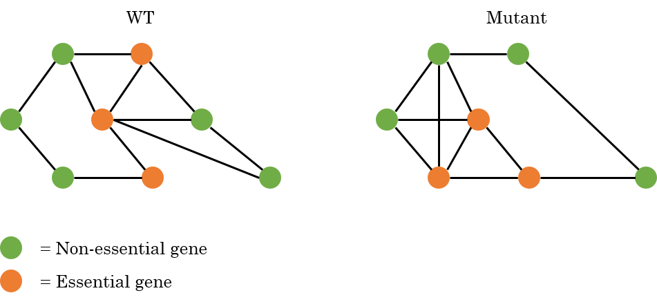
The idea is that the essentiality of genes (both type I and type II), may change between different genetic backgrounds. For changes in essentiality four cases are considered:
A gene is essential in WT and remains essential in the mutant.
A gene is non-essential in WT and remains non-essential in the mutant.
A gene is essential in WT and becomes non-essential in the mutant.
A gene is non-essential in WT and becomes essential in the mutant.
An example is given in the figure below, where an interaction map is shown for WT cells and a possible interaction map for a mutant where both the essentiality and the interactions are changed.
Situation 1 and 3 are expected to be the trickiest since those ones are difficult to validate. To check the synthetic lethality in cells, a double mutation needs to be made where one mutation makes the genetic background and the second mutation should confirm whether the second mutated gene is actually essential or not. This is typically made by sporulating the two mutants, but deleting a gene that is already essential in wild type prevents the cell from growing or dividing and can therefore not be sporulated with the mutant to create the double deletion. Therefore, these double mutants are hard or impossible to make.
Another point to be aware of is that some genes might be essential in specific growth conditions (see also the subsection). For example, cells that are grown in an environment that is rich of a specific nutrient, the gene(s) that are required for the digestion of this nutrient might be essential in this condition. The SATAY experiments will therefore show that these genes are intolerant for transposon insertions. However, when the cells are grown in another growth condition where mainly other nutrients are present, the same genes might now not be essential and therefore also be more tolerant to transposon insertions in that region. It is suggested to compare the results of experiments with cells from the same genetic background grown in different conditions with each other to rule out conditions specific results.
We want to check the essentiality of all genes in different mutants and compare this with both wild type cells and with each other. The goal is to make an overview of the changes in the essentiality of the genes and the interaction network between the proteins. With this we aim to eventually be able to predict the synthetic lethality of multiple mutations based on the interaction maps of the individual mutations.
Interpreting Transposon Counts & Reads¶
Once cells have a transposon inserted somewhere in the DNA, the cells are let to grow so they can potentially generate a few new generations. A cell with a transposon inserted in an essential part of its DNA grows very slowly or might not grow at all (due to its decreased fitness). Since the sequencing starts only at the location of a transposon insertion (see experimental methods section), it can be concluded that roughly each read from the sequencing corresponds with a transposon insertion (roughly mainly because transposon inserted in essential genes can generate no reads). Cells with a transposon inserted in an essential genomic region, will not have divided and therefore will not have a contribution to the sequencing reads. When the reads are aligned to a reference sequence and the number of reads are mapped against the genome, empty regions indicate possible essential genes. Negative selection can thus be found by looking for empty regions in the reads mapping. When a transposon is inserted in a non-essential genomic region, these cells can still divide and give rise to offspring and after sequencing the non-essential regions will be represented by relatively many reads.
During processing the genes can be analysed using the number of transposon insertions per gene (or region) or the number of reads per gene. Reads per gene, instead of transposons per gene, might be a good measure for positive selection since it is more sensitive (bigger difference in number of reads between essential and non-essential genes), but also tends to be nosier. Transposons per gene is less noisy, but is also less sensitive since the number of transposons inserted in a gene does not change in subsequent generations of a particular cell. Therefore it is hard to tell the fitness of cells when a transposon is inserted a non-essential region solely based on the number of transposon insertions.
Ideally only the transposons inserted in non-essential genomic regions will have reads (since only these cells can create a colony before sequencing), creating a clear difference between the essential and non-essential genes. However, sometimes non-essential genes also have few or no transposon insertion sites. According to Michel et.al. this can have 3 main reasons.
During alignment of the reads, the reads that represent repeated DNA sequences are discarded, since there is no unique way of fitting them in the completed sequence. (Although the DNA sequence is repeated, the number of transposon counts can differ between the repeated regions) Transposons within such repeated sequences are therefore discarded and the corresponding reads not count. If this happens at a non-essential gene, it appears that it has no transposons, but this is thus merely an alignment related error in the analysis process.
Long stretches of DNA that are without stop codons, called Open Reading Frames (ORF), typically code for proteins. Some dubious ORF might overlap with essential proteins, so although these ORF themselves are not essential, the overlapping part is and therefore they do not show any transposons.
Some genes are essential only in specific conditions. For example, genes that are involved in galactose metabolism are typically not essential, as inhibition of these genes block the cell’s ability to digest galactose, but it can still survive on other nutrition’s. In lab conditions however, the cells are typically grown in galactose rich media, and inhibiting the genes for galactose metabolism cause starvation of the cells.
A gene might not be essential, but its deletion might cripple the cell so that the growth rate decreases significantly. When the cells are grown, the more healthy cells grow much faster and, after some time, occur more frequently in the population than these crippled cells and therefore these cells might not generate many reads or no reads at all. In the processing, it might therefore look as if these genes are essential, but in fact they are not. The cells just grow very slowly.
The other way around might also occur, where essential genes are partly tolerant to transposons. This is shown by Michel et.al. to be caused that some regions (that code for specific subdomains of the proteins) of the essential genes are dispensable. The transposons in these essential genes are clearly located at a specific region in the gene, the one that codes for a non-essential subdomain. However, this is not always possible, as in some cases deletion of non-essential subdomains of essential genes create unstable, unexpressed or toxin proteins. The difference in essentiality between subdomains in a single protein only happens in essential genes, not in non-essential genes. Michel et.al. devised an algorithm to estimate the likelihood \(L\) of a gene having an essential subdomain:
where \(d\) is the longest interval (in terms of base pairs) between 5 neighbouring transposons in a Coding DNA Sequence (cds) (\(\geq 300\) bp), \(N_{cds}\) is the total number transposons mapping in the cds (\(\geq 20\)) transposons) and \(l_{cds}\) is the total length of the CDS. Additionally, it must hold that \(0.1 l_{cds} \leq d \leq 0.9 l_{cds}\).
It is expected that only essential genes carry essential subdomains, and indeed what was found by Michel et.al. that the genes with the highest likelihood were mostly also genes previously annotated as essential by other studies.
Because of the reasons mentioned before, not a simple binary conclusion can be made solely based on the amount of transposon insertions or the number of reads. Instead, a gene with little reads might be essential, but to be sure the results from other experiments need to be implemented as well, for example where the cells were grown in a different growth conditions. Therefore, SATAY analysis only says something about the relative fitness of cells where a specific gene is inhibited in the current growth conditions.
Quality check
Comparison of our results with those obtained by the Kornmann lab might confirm the quality of our experimental and analysis methods. PUT FIGURE
Experimental Process¶
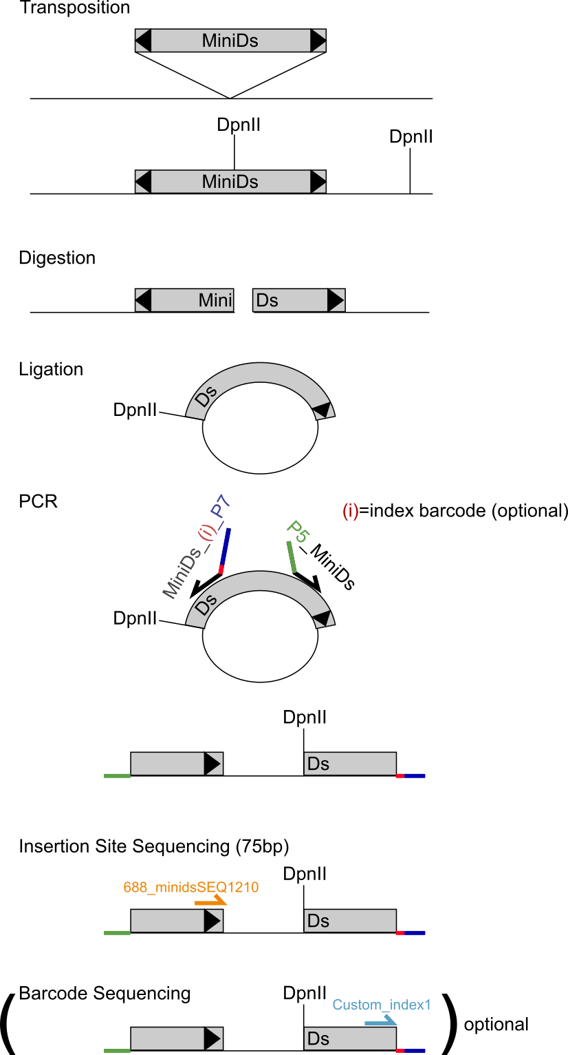
The process of SATAY starts with inserting a plasmid in the cells that contains a transposase (TPase) and the transposon (MiniDs) flanked on both sides by adenine (ADE). The transposon has a specific, known, sequence that codes for the transposase that cuts the transposon from the plasmid (or DNA) to (another part of) the DNA.
Simplified example for the transposon insertion plasmid.
The MiniDs transposon is cut loose from the plasmid and randomly inserted in the DNA of the host cell.
If the transposon is inserted in a gene, the gene can still be transcribed by the ribosomes, but typically cannot be (properly) translated in a functional protein.
The genomic DNA (with the transposon) is cut in pieces for sequencing using enzymes, for example DpnII.
This cuts the DNA in many small pieces (e.g. each 75bp long) and it always cuts the transposon in two parts (i.e. digestion of the DNA).
Each of the two halves of the cut transposon, together with the part of the gene where the transposon is inserted in, is ligated meaning that it is folded in a circle.
A part of the circle is then the half transposon and the rest of the circle is a part of the gene where the transposon is inserted in.
Using PCR and primers, this can then be unfolded by cutting the circle at the halved transposon.
The part of the gene is then between the transposon quarters.
Since the sequence of the transposon is known, the part of the gene can be extracted.
This is repeated for the other half of the transposon that includes the other part of the gene.
When both parts of the gene are known, the sequence from the original gene can be determined.
Sequence alignment¶
To get the order of nucleotides in a genome, shotgun sequencing is used where the genome is cut is small pieces called reads (typically tens to a few hundred basepairs long).
The reads have overlapping regions that can be used to identify their location with respect to a reference genome and other reads (i.e. mapping of the reads).
Mapping of the reads result in contigs, which are multiple mapped reads that form continuous assembled parts of the genome (contigs can be the entire target genome itself).
All contigs should be assembled to form (a large part of) the target genome.
The sequence assembly problem can be described as: Given a set of sequences, find the minimal length string containing all members of the set as substrings.
The reads from the sequencing can be single-end or paired-end, which indicates how the sequencing is performed. In paired-end sequencing, the reads are sequenced from both directions, making the assembly easier and more reliable, but results in twice as many reads as single-end reads. The reason of the more reliable results has to do with ambiguous reads that might occur in the single-end sequencing. Here, a read can be assigned to two different locations on the reference genome (and have the same alignment score). In these cases, it cannot be determined where the read should actually be aligned (hence its position is ambiguous). In paired-end sequencing, each DNA fragment has primers on both ends, meaning that the sequencing can start in both the 5’-3’ direction and in the 3’-5’ direction. Each DNA fragment therefore has two reads both which have a specified length that is shorter than the entire DNA fragment. This results that a DNA fragment is read on both ends, but the central part will still be unknown (as it is not covered by these two particular reads, but it will be covered by other reads). Since you know that the two reads belong close together, the alignment of one read can be checked by the alignment of the second read (or paired mate) somewhere in close vicinity on the reference sequence. This is usually enough for the reads to become unambiguous.
The resulting data from the sequencing is stored in a FASTQ file where all individual reads are stored including a quality score of the sequencing. The reads are in random order and therefore the first step in the processing is aligning of the reads in the FASTQ files with a reference genome.
Note that the quality of the reads typically decreases near the 3’-end of the reads due to the chemistry processes required for sequencing (this depends on the kind of method used). For Illumina sequencing, the main reasons are signal decay and dephasing, both causing a relative increase in the background noise. Dephasing occurs when a DNA fragment is not de-blocked properly. A DNA fragment is copied many times and all copies incorporate a fluorescent nucleotide that can be imaged to identify the nucleotide. If there are 1000 copies of the DNA fragment, there are 1000 fluorescent nucleotides that, ideally, are all the same to create a high quality signal. After imaging, the DNA fragment is de-blocked to allow a new fluorescent nucleotide to bind. This deblocking might not work for all copies of the DNA fragment. For example, 100 copies might not be deblocked properly, so for the next nucleotide only 900 copies agree for the next incorporated nucleotide. For the third round, the 100 copies that were not deblocked properly in the second round, might now be deblocked as well, but now they are lagging behind one nucleotide, meaning that in the coming rounds they have consistently the wrong nucleotide. As the reads increases in length, more rounds are needed and therefore the chances of dephasing increases causing a decrease in the quality of the reads. This gives noise in the signal of the new nucleotide and therefore the quality of the signal decreases. For example, take the next 6bp sequence that is copied 5 times:
GATGTCGATGTCG ATGTGAT GTG AT G
The first two reads are deblocked properly and they give all the right nucleotides. But the third and fourth have one round that is not deblocked properly (indicated by the empty region between the nucleotides), hence the nucleotide is always lagging one bp after the failed deblocking. The fifth copy has two failed deblocking situations, hence is lagging two bp. The first nucleotide is a G for all 5 copies, therefore the quality of this nucleotide is perfect. But, by the end of the read, only two out of five copies have the correct bp (i.e. a C), therefore the quality is poor for this nucleotide. (It can either be a C or a T with equal likelyhood or potentially a G, so determining which nucleotide is correct is ambiguous without knowing which reads are lagging, which you don’t know). (See for example this question on seqanswers or the paper by [Pfeifer, 2016])
File Types¶
fastq¶
This is the standard output format for sequencing data. It contains all (raw) sequencing reads in random order including a quality string per basepair. Each read has four lines:
Header: Contains some basic information from the sequencing machine and a unique identifier number.
Sequence: The actual nucleotide sequence.
Dummy: Typically a ‘+’ and is there to separate the sequence line from the quality line.
Quality score: Indicates the quality of each basepair in the sequence line (each symbol in this line belongs to the nucleotide at the same position in the sequence line). The sequence and this quality line should always have the same length.
The quality line is given as a phred score. There are two versions, base33 and base64, but the base64 is outdated and hardly used anymore. In both versions the quality score is determined by Q = -10*log10§ where P is the error probability determined during sequencing (0 < P < 1). A Q-score of 0 (i.e. an error probability of P=1) is defined by ascii symbol 33 (‘!’) for base33 and by ascii symbol 64 (‘@’) for base64. A Q-score of 1 (p=0.79) is then given by ascii 34 (’ ” ‘) (for base33) etcetera. For a full table of ascii symbols and probability scores, see the appendices of this document PHRED table (base33) and PHRED table (base64). Basically all fastq files that are being created on modern sequencing machines use the base33 system.
The nucleotide sequence typically only contains the four nucleotide letters (A, T, C and G), but when a nucleotide was not accurately determined (i.e. having a error probability higher than a certain threshold), the nucleotide is sometimes converted to the letter N, indicating that this nucleotide was not successfully sequenced.
Fastq files tend to be large in size (depending on how many reads are sequenced, but >10Gb is normal). Therefore these files are typically compressed in gzip format (.fastq.gz). The pipeline can handle gzipped files by itself, so there is no need to convert it manually.
Example fastq file:
@NB501605:544:HLHLMBGXF:1:11101:9938:1050 1:N:0:TGCAGCTA
TGTCAACGGTTTAGTGTTTTCTTACCCAATTGTAGAGACTATCCACAAGGACAATATTTGTGACTTATGTTATGCG
+
AAAAAEEEEEEEEEEEEEEEEEEEEEEEEEEEEEEEEEEEEEEEEEEEEEEEEEEEEEEEEEEEEEEEEEEEEEE
@NB501605:544:HLHLMBGXF:1:11101:2258:1051 1:N:0:TACAGCTA
TGAGGCACCTATCTCAGCGATCGTATCGGTTTTCGATTACCGTATTTATCCCGTTCGTTTTCGTTGCCGCTATTT
+
AAAAAEEEEEEEEEEEEEEEEEEEEEEEEEEEEEEEEEEEEEEE6EEEEEEEE<EEEAEEEEEEE/E/E/EA///
@NB501605:544:HLHLMBGXF:1:11101:26723:1052 1:N:0:TGCAGCTA
TGTCAACGGTTTAGTGTTTTCTTACCCAATTGTAGAGACTATCCACAAGGACAATATTTGTGACTTATGTTATGCG
+
AAAAAEEEEEEEEEEEEEEEEEEEEEEEEEEEEEEEEEEEEEEEEEEEEEEEEEEEEEEEEEEEEEEEEEEEEEEE
sam, bam¶
When the reads are aligned to a reference genome, the resulting file is a Sequence Alignment Mapping (sam) file. Every read is one line in the file and consists of at least 11 tab delimited fields that are always in the same order:
Name of the read. This is unique for each read, but can occur multiple times in the file when a read is split up over multiple alignments at different locations.
Flag. Indicating properties of the read about how it was mapped (see below for more information).
Chromosome name to which the read was mapped.
Leftmost position in the chromosome to which the read was mapped.
Mapping quality in terms of Q-score as explained in the fastq section.
CIGAR string. Describing which nucleotides were mapped, where insertions and deletions are and where mismatches occurs. For example,
43M1I10M3D18Mmeans that the first 43 nucleotides match with the reference genome, the next 1 nucleotide exists in the read but not in the reference genome (insertion), then 10 matches, then 3 nucleotides that do not exist in the read but do exist in the reference genome (deletions) and finally 18 matches. For more information see this website.Reference name of the mate read (when using paired end datafiles). If no mate was mapped (e.g. in case of single end data or if it was not possible to map the mate read) this is typically set to
*.Position of the mate read. If no mate was mapped this is typically set to
0.Template length. Length of a group (i.e. mate reads or reads that are split up over multiple alignments) from the left most base position to the right most base position.
Nucleotide sequence.
Phred score of the sequence (see fastq section).
Depending on the software, the sam file typically starts with a few header lines containing information regarding the alignment.
For example for BWA MEM (which is used in the pipeline), the sam file start with @SQ lines that shows information about the names and lengths for the different chromosome and @PG shows the user options that were set regarding the alignment software.
Note that these lines might be different when using a different alignment software.
Also, there is a whole list of optional fields that can be added to each read after the first 11 required fields.
For more information, see wikipedia.
The flag in the sam files is a way of representing a list of properties for a read as a single integer. There is a defined list of properties in a fixed order:
read paired
read mapped in proper pair
read unmapped
mate unmapped
read reverse strand
mate reverse strand
first in pair
second in pair
not primary alignment
read fails platform/vendor quality checks
read is PCR or optical duplicate
supplementary alignment
To determine the flag integer, a 12-bit binary number is created with zeros for the properties that are not true for a read and ones for those properties that are true for that read. This 12-bit binary number is then converted to a decimal integer. Note that the binary number should be read from right to left. For example, FLAG=81 corresponds to the 12-bit binary 000001010001 which indicates the properties: ‘read paired’, ‘read reverse strand’ and ‘first in pair’. Decoding of sam flags can be done using this website or using samflag.py.
Example sam file (note that the last read was not mapped):
NB501605:544:HLHLMBGXF:1:11101:25386:1198 2064 ref|NC_001136| 362539 0 42H34M * 0 0 GATCACTTCTTACGCTGGGTATATGAGTCGTAAT EEEAEEEEEEAEEEAEEAEEEEEEEEEEEAAAAA NM:i:0 MD:Z:34 AS:i:34 XS:i:0 SA:Z:ref|NC_001144|,461555,+,30S46M,0,0;
NB501605:544:HLHLMBGXF:1:11101:20462:1198 16 ref|NC_001137| 576415 0 75M * 0 0 CTGTACATGCTGATGGTAGCGGTTCACAAAGAGCTGGATAGTGATGATGTTCCAGACGGTAGATTTGATATATTA EEEAEEEEEEEEEEEEEAEEAE/EEEEEEEEEEEAEEEEEE/EEEEEAEAEEEEEEEEEEEEEEEEEEEEAAAAA NM:i:1 MD:Z:41C33 AS:i:41 XS:i:41
NB501605:544:HLHLMBGXF:1:11101:15826:1199 4 * 0 0 * * 0 0 ACAATATTTGTGACTTATGTTATGCG EEEEEEEEEEE6EEEEEEEEEEEEEE AS:i:0 XS:i:0
Sam files tend to be large in size (tens of Gb is normal).
Therefore the sam files are typically stored as compressed binary files called bam files.
Almost all downstream analysis tools (at least all tools discussed in this document) that need the alignment information accept bam files as input.
Therefore the sam files are mostly deleted after the bam file is created.
When a sam file is needed, it can always be recreated from the bam file, for example using SAMTools using the command samtools view -h -o out.sam in.bam.
The bam file can be sorted (creating a .sorted.bam file) where the reads are typically ordered depending on their position in the genome.
This usually also comes with an index file (a .sorted.bam.bai file) which stores some information where for example the different chromosomes start within the bam file and where specific often occuring sequences are.
Many downstream analysis tools require this file to be able to efficiently search through the bam file.
bed¶
A bed file is one of the outputs from the transposon mapping pipeline.
It is a standard format for storing read insertion locations and the corresponding read counts.
The file consists of a single header, typically something similar to track name=[file_name] userscore=1.
Every row corresponds to one insertion and has (in case of the satay analysis) the following space delimited columns:
chromosome (e.g.
chrIorchrref|NC_001133|)start position of insertion
end position of insertion (in case of satay-analysis, this is always start position + 1)
dummy column (this information is not present for satay analysis, but must be there to satisfy the bed format)
number of reads at that insertion location
In case of processing with transposonmapping.py (final step in processing pipeline) or the matlab code from the kornmann-lab, the number of reads are given according to (reads*20)+100, for example 2 reads are stored as 140.
The bed file can be used for many downstream analysis tools, for example genome_browser.
Sometimes it might occur that insertions are stored outside the chromosome (i.e. the insertion position is bigger than the length of that chromosome).
Also, reference genomes sometimes do not have the different chromosomes stored as roman numerals (for example chrI, chrII, etc.) but rather use different names (this originates from the chromosome names used in the reference genome).
These things can confuse some analysis tools, for example the genome_browser.
To solve this, the python function clean_bedwigfiles.py is created.
This creates a _clean.bed file where the insertions outside the chromosome are removed and all the chromosome names are stored with their roman numerals.
See clean_bedwigfiles.py for more information.
Example bed file:
track name=leila_wt_techrep_ab useScore=1
chrI 86 87 . 140
chrI 89 90 . 140
chrI 100 101 . 3820
chrI 111 112 . 9480
wig¶
A wiggle (wig) file is another output from the transposon mapping pipeline.
It stores similar information as the bed file, but in a different format.
This file has a header typically in the form of track type=wiggle_0 maxheightPixels=60 name=[file_name].
Each chromosome starts with the line variablestep chrom=chr[chromosome] where [chromosome] is replaced by a chromosome name, e.g. I or ref|NC_001133|.
After a variablestep line, every row corresponds with an insertion in two space delimited columns:
insertion position
number of reads
In the wig file, the read count represent the actual count (unlike the bed file where an equation is used to transform the numbers).
There is one difference between the bed and the wig file. In the bed file the insertions at the same position but with a different orientation are stored as individual insertions. In the wig file these insertions are represented as a single insertion and the corresponding read counts are added up.
Similar to the bed file, also in the wig insertions might occur that have an insertion position that is bigger then the length of the chromosome. This can be solved with the same python script as the bed file. The insertions that have a position outside the chromosome are removed and the chromosome names are represented as a roman numeral.
Example wig file:
track type=wiggle_0 maxheightPixels=60 name=WT_merged-techrep-a_techrep-b_trimmed.sorted.bam
variablestep chrom=chrI
86 2
89 2
100 186
111 469
pergene.txt, peressential.txt¶
A pergene.txt and peressential.txt file are yet another outputs from the transposon mapping pipeline. Where bed and wig files store all insertions throughout the genome, these files only store the insertions in each gene or each essential gene, respectively. Essential genes are the annotated essential genes as stated by SGD for wild type cells. The genes are taken from the Yeast_Protein_Names.txt file, which is downloaded from uniprot. The positions of each gene are determined by a gff3 file downloaded from SGD. Essential genes are defined in Cerevisiae_AllEssentialGenes.txt.
The pergene.txt and the peressential.txt have the same format. This consists of a header and then each row contains three tab delimited columns:
gene name
total number of insertions within the gene
sum of all reads of those insertions
The reads are the actual read counts. To suppress noise, the insertion with the highest read count in a gene is removed from that gene. Therefore, it might occur that a gene has 1 insertion, but 0 reads.
Note that when comparing files that include gene names there might be differences in the gene naming. Genes have multiple names, e.g. systematic names like ‘YBR200W’ or standard names like ‘BEM1’ which can have aliases such as ‘SRO1’. The above three names all refer to the same gene. The Yeast_Protein_Names.txt file can be used to search for aliases when comparing gene names in different files.
Example of pergene.txt file:
Gene name Number of transposons per gene Number of reads per gene
YAL069W 34 1819
YAL068W-A 10 599
PAU8 26 1133
YAL067W-A 12 319
pergene_insertions.txt, peressential_insertions.txt¶
The final two files that are created by the transposon mapping pipeline are the pergene_insertions.txt and the peressential_insertions.txt. The files have a similar format as the pergene.txt file, but are more extensive in terms of the information per gene. The information is taken from Yeast_Protein_Names.txt, the gff3 file and Cerevisiae_AllEssentialGenes.txt, similar as the pergene.txt files.
Both the pergene_insertions.txt and the peressential_insertions.txt files have a header and then each row contains six tab delimited columns:
gene name
chromosome where the gene is located
start position of the gene
end position of the gene
list of all insertions within the gene
list of all read counts in the same order as the insertion list
This file can be useful when not only the number of insertions is important, but also the distribution of the insertions within the genes. Similarily as the pergene.txt and peresential.txt file, to suppress noise the insertion with the highest read count in a gene is removed from that gene.
This file is uniquely created in the processing workflow described below.
If the index file .bam.bai is not present, create this before running the python script. The index file can be created using the command
sambamba-0.7.1.-linux-static sort -m 1GB [path]/[filename.bam]. This creates a sorted.bam file and a sorted.bam.bai index file.
Example of peressential_insertions.txt file:
EFB1 I 142174 143160 [142325, 142886] [1, 1]
PRE7 II 141247 141972 [141262, 141736, 141742, 141895] [1, 1, 1, 1]
RPL32 II 45978 46370 [46011, 46142, 46240] [1, 3, 1]
Determine essentiality based on transposon counts¶
Using the number of transposons and reads, it can be determined which genes are potentially essential and which are not.
To check this method, the transposon count for wild type cells are determined. Currently, genes that are taken as essential are the annotated essentials based on previous research.
We can use statitiscal learning methods to find what is the expected number of transposons per essential gene. See this Matlab Code done by one of our Master students in our lab, Wessel Teunisse.
Distribution number of insertions and reads compared with essential and non-essential genes¶
Ideally, the number of transposon insertions of all essential genes are small and the number of insertions in non-essential genes are is large so that there is a clear distinction can be made. However, this is not always so clear. For example, the distribution of transposons in WT cells in the data from Michel et. al. looks like this:
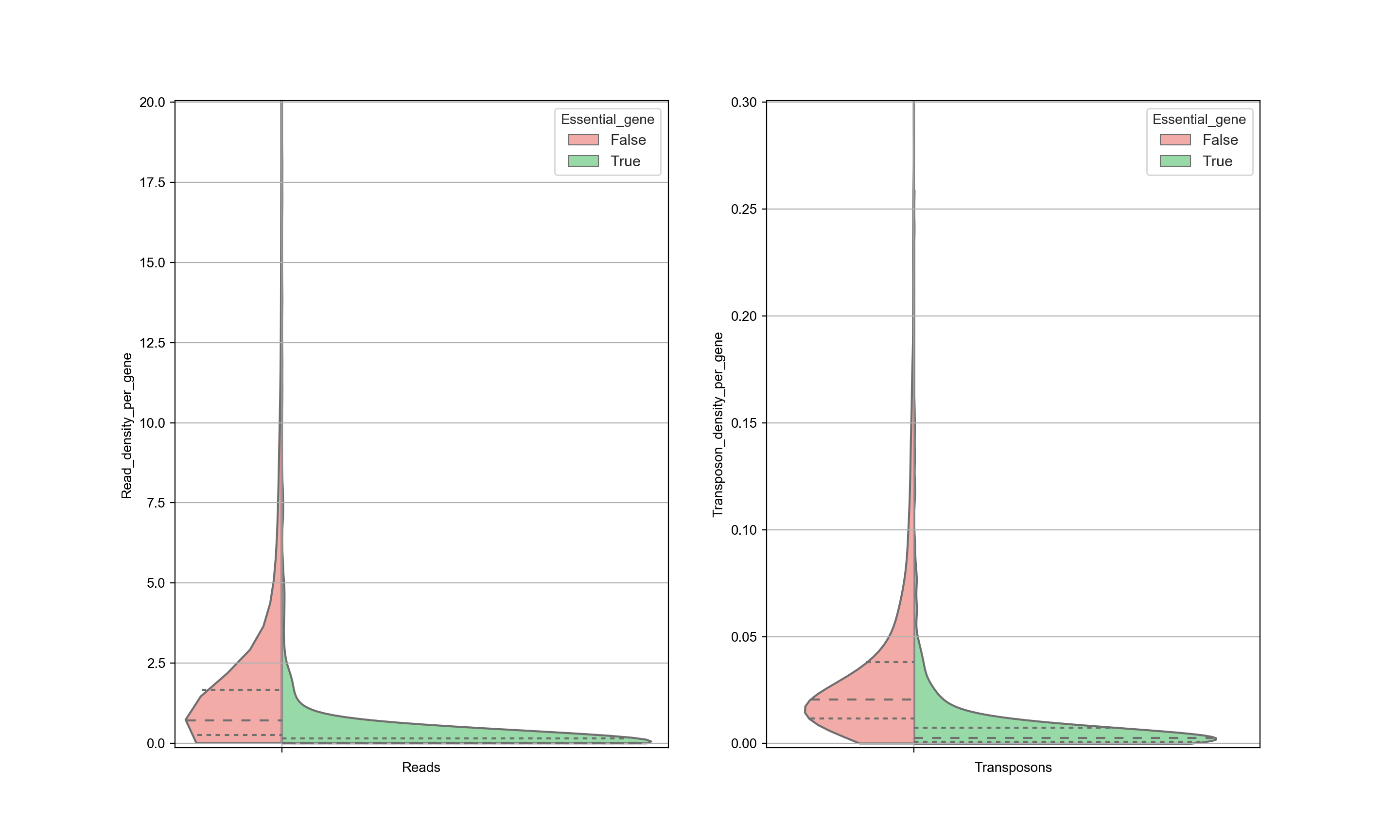
In this figure, both the reads and the transposon counts are normalized with respect to the length of each gene (hence the graph represents the read density and transposon density). High transposon counts only occurs for non-essential genes, and therefore when a high transposon count is seen, it can be assigned nonessential with reasonable certainty. However, when the transposon count is low the there is a significant overlap between the two distributions and therefore there is no certainty whether this gene is essential or not (see also the section about ‘Interpreting Transposon Counts & Reads’).
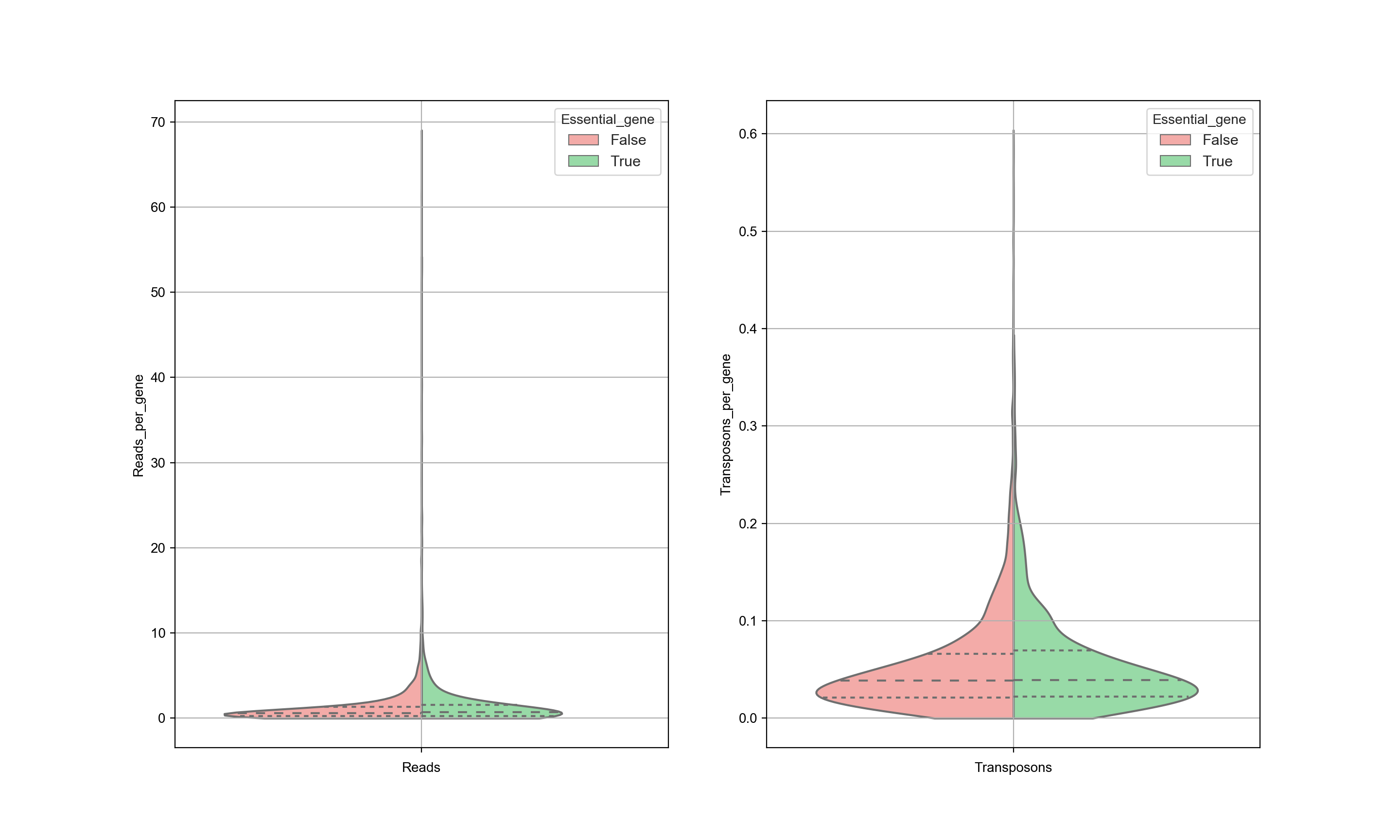
The data is also sensitive to postprocessing. It is expected that the trimming of the sequences is an important step. The graph below shows the same data as in the previous graph, but with different processing as is done by Michel et. al… This has a significant influence on the results and as a consequence, no distinction can be made between essential and nonessential genes based on the transposon counts. Significant attention needs to be given to the postprocessing of the data.
Profile plot for number of reads¶
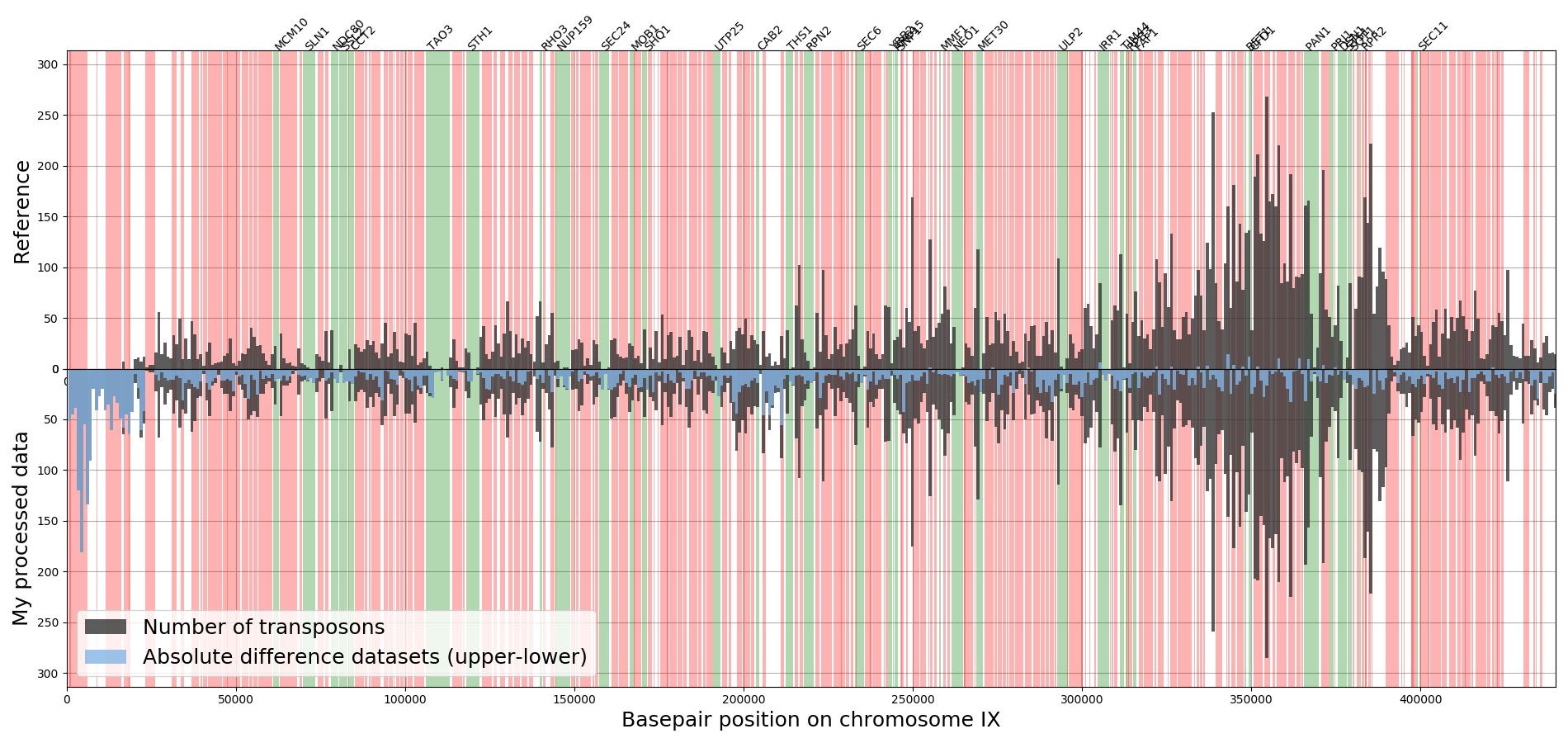
To create a visual overview where the insertions are and how many reads there are for each insertion, a profile plot is created for each chromosome.
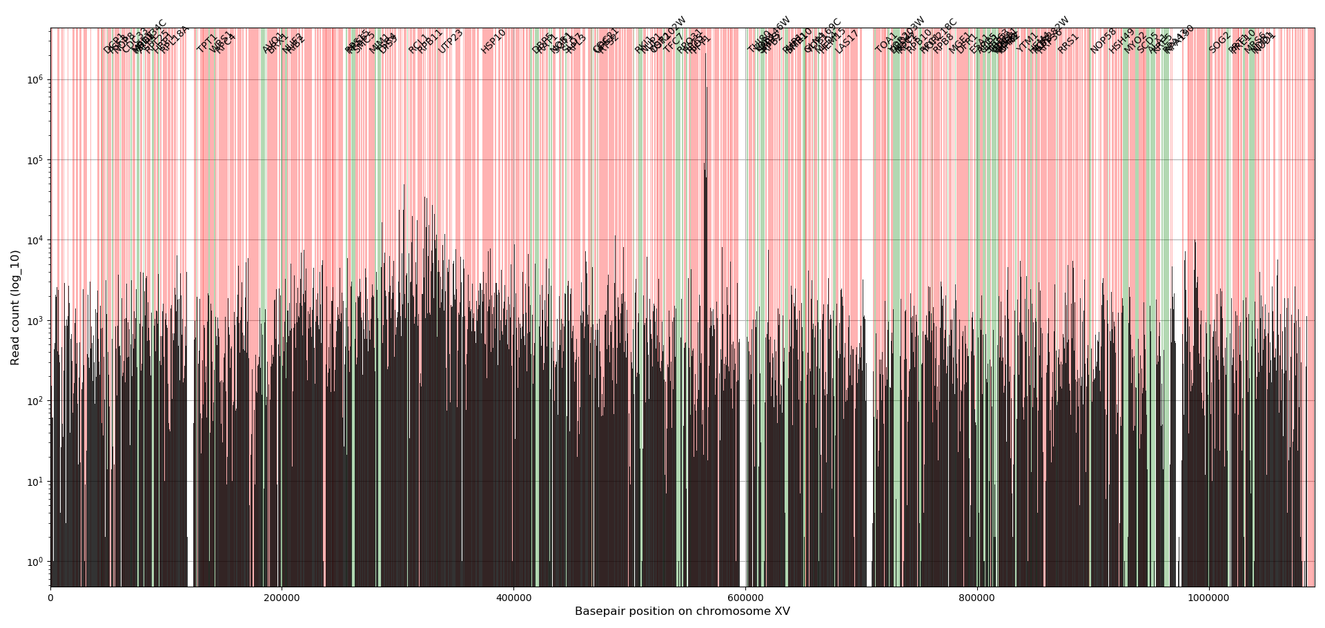
The bars indicate the absolute number of reads for all insertions located in the bars (bar width is 545bp). The colored background indicate the location of genes, where green are the annotated essential genes and red the non-essential genes. In general, the essential genes have no or little reads whereas the non-essential genes have many reads. Note that at location 564476 the ADE2 gene is located that has significant more reads than any other location in the genome, which has to do the way the plasmid is designed (see Michel et.al. 2017). The examples used here are from a dataset discussed in the paper by Michel et.al. 2017 which used centromeric plasmids where the transposons are excised from. The transposons tend to reinsert in the chromosome near the chromosomal pericentromeric region causing those regions to have about 20% more insertions compared to other chromosomal regions.
This figure gives a rough overview that allows for identifying how well the data fits the expectation.
Also an alternative version of this plot is made (TransposonRead_Profile_Compare.py) that makes a similar plot for two datasets at the same time, allowing the comparison of the two datasets with each other and with the expectation.